Introduction
Since the invention of calculus and Newton’s Principia, ODEs and PDEs (Ordinary / Partial Differential Equations) have been the most used class of models for natural phenomena. The laws of Newton and Kepler are ODEs, fluid mechanics and electromagnetism are modeled using PDEs. So are elasticity, plasticity, thermodynamics, quantum mechanics, or climate models. The examples are innumerable and can be found across all science and engineering, and they have driven the development and construction of ever more powerful supercomputers. The efficient solution of DEs is key to the advancement of science and its successful application in engineering.
The two problems
The application of neural networks to DEs has a long history: long after seminal works like [Dis94N] and [Lag98A, Lag00N] interest has currently rekindled, motivated by the successes of NNs in computer vision, natural language processing and other fields. We can distinguish two main tasks to solve:
In the direct problem, given a PDE $L(u)=f$ with known coefficients, domain and initial and boundary conditions, one wishes to compute or approximate a solution. The simplest approach, which we consider below, is to directly minimise the MSE $||L(\hat u) - f||_2^2$, with some additional terms.
In the inverse problem, a parametrised PDE is given, and some values of the solution are observed. The task (system identification), is then to infer the parameters of the equation governing the system [Rai18H, Rai19P]. A related line of research learns the structure of the equations instead of just the coefficients. Some do a form of symbolic regression defined by activation functions [Sah18L]. [Lon18P] shows how differential operators are approximated by convolution filters and learns those. Some techniques are meta-heuristic, others use gradient-based approaches [Bru16D, Qin19D].
In this note, we focus on the direct problem and a family of methods tackling it.
The curse of dimensionality
The dimension of the solution for most DEs grows quickly with the size of the system. For example, in ab-initio molecular dynamics, every atom is represented as a point described by 6 numbers (3 position coordinates, 3 velocity coordinates). Consequently, the dimension of the system grows like $6N$. In this field, the simulation of a small drop of water is a traditional benchmark since it acts as solvent in many systems, and one can quickly verify how such a “simple problem” can become untractable with hexabyte storage and other impossible requirements.1 1 To comprehend the extent of the problem, consider the following back-of-the-napkin calculation. The molar mass of water is 18 g/mol, so one drop contains around $5 \cdot 10^{-4}$ mol of water, or $3.34 \cdot 10^{20}$ molecules. Each molecule is made of 3 atoms, 2H and O, so there will be $N = 10^{21}$ atoms. Making the optimistic assumption that position and velocity vectors of each atom are enough to describe the system (disregarding interactions, among other things), we need $6 \cdot N$ numbers, which, using 32-bit precision, roughly amounts to $2.4 \cdot 10^{22}$ bytes. That is, 21 billion terabytes are needed in order to store a snapshot of the system. Of course, there are macro descriptions of the behaviour of water but that is besides the point. For one thing, when using ab-initio techniques, some of the properties of water ( hydrogen bonds, capillarity, etc) emerge naturally. The important point, however, is that the number of molecules is huge. Its lower range is in the thousands and its higher range around Avogadro’s number ($10^{23}$). Furthermore, most molecules of interest have many more atoms than water, e.g. penicillin is made of 41 atoms and proteins can have thousands of them.
As an example, the figure below shows how the dimension of the solution of Schrödinger’s equation grows with the size of the molecule being simulated.
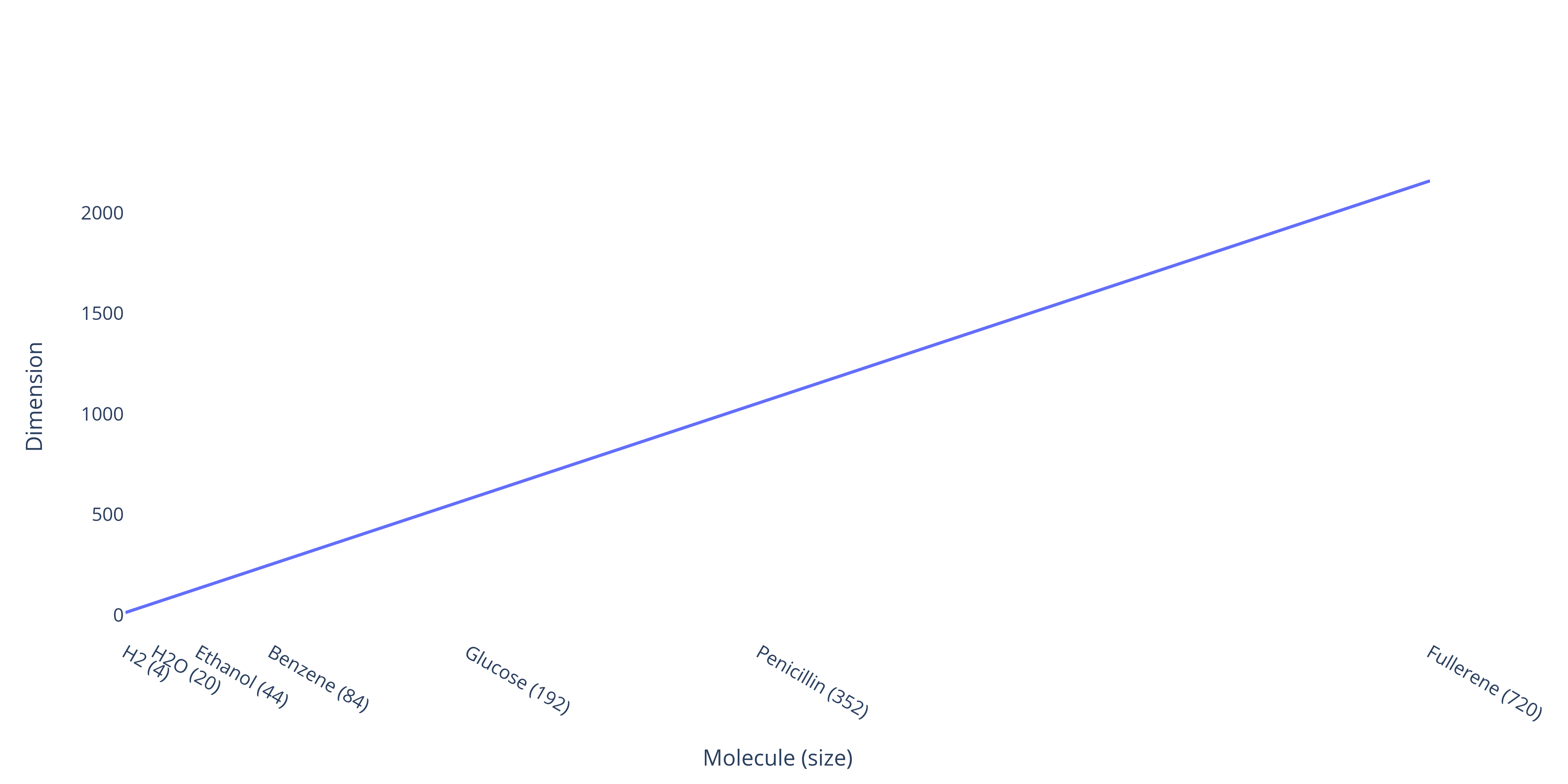
Dimension scaling of Schrödinger's equation
This plot is for just one molecule of each compound. Most simulations of practical relevance will have billions of molecules.
This is further aggravated by the grids which methods like FEM or Finite Differences (FD) use. Due to the curse of dimensionality, the number of grid points also grows exponentially. In some cases, solution quality can be traded for computational requirements by using coarse or adaptive grids, but even that tradeoff has limits. Some systems just grow too fast.
One advantage of approximating the solutions as a NN instead of as values on a grid is that we can dispense with the grid altogether. This, at least in theory, could open the door to dealing with high-dimensional problems that were previously intractable.
Solving the direct problem
There are a number of approaches to incorporating NNs in the solution procedures of DEs. [Dea18E] introduce an end-to-end differential physics simulator that can be used to allow full back-propagation and improve the performance of algorithms that use it. [Um21S] solve equations using traditional, grid-based solvers on a coarse grid and use a NN to add a fine correction term to the coarse solution. As specifying the grid upon which to solve the equation is a non-trivial task, [Bar19L] learn it instead. [Rai18H] uses not neural networks but a Gaussian Process prior on the solutions. [Lad15D] use regression forests to simulate fluids and [Li20F] attempt to learn the solution operator.
We will examine Physically Inspired Neural Networks (PINNs) [Rai19P] and Deep Galerkin Methods (DGM) [Sir18D] in detail, a family of methods that instead of using linear combinations of basis vectors like in FEM, represent the solution as a NN. This has been an active area of research recently [Han18S, Kha19V, Shi20C, Lu21L]. In order to find the best approximation to the solution, one has to solve a non-linear optimization problem. Recall that a solution to a PDE is a function that fulfills all the equation’s conditions, i.e. the equation proper, the boundary conditions, and the initial conditions. A loss function that measures how much the NN violates the equation constraints can be specified and then minimized, as we can numerically evaluate the differential operator applied to the network. If we add initial and boundary conditions, then achieving a zero loss means obtaining one solution. Of course, in practice zero is never perfectly attained, but a network with low enough loss can be a satisfactory solution.
Avoiding the curse of dimensionality: the PINN / DGM method
Even though it has appeared independently under two names in the literature, PINN and DGM, the underlying method is essentially the same. The main component of PINN [Rai19P] and DGM [Sir18D] is an appropriately crafted loss function that measures how far the network is from the solution to the problem. All the information we need is contained in the equation itself, and the additional conditions that a solution has to fulfill. We just need to measure how far the current network is from fulfilling them. Therefore, we construct a composite loss
$$L = L_s +L_b + L_i$$
where the subscript $s$ stands for structural, $b$ for boundary and $i$ for initial. Let us use the heat equation, a canonical example, to illustrate our definitions. Let $\Omega \subset \mathbb{R}$ be an open, bounded subinterval of the real line and let $t \in \mathbb{R}$ denote time. The 1-dimensional heat equation is given by
$$\Delta u (t, x) = \frac{\partial u(t, x)}{\partial t}, t \in \mathbb{R}, x \in \Omega.$$
Now, each of the sub-losses is defined as:
$$\displaylines{L_{structural} = \frac{1}{N_{r}} \sum \left(\Delta u - \frac{\partial u}{\partial t}\right)^2 \\ L_{boundary} = \frac{1}{N_{b}} \sum (u - g)^2 \\ L_ {initial} =\frac{1}{N_{i}} \sum (u - u_0)^2}$$
In the above, $g(t, x)$ is a given boundary condition, defined for all $t\in\mathbb{R}$ and $x \in \partial \Omega$, the boundary of $\Omega$, and $u_0(x)$ is the initial condition, given over all of $\Omega$.
Note that we measure each loss only within its domain. That is, the initial loss only over points with $t = 0$, the boundary loss only on the boundary (i.e. $ x \in \partial \Omega$) and the structural loss on the rest of the domain. The points can be sampled in multiple ways. Both fixed and adaptive grids could be used, but the main advantage of these methods is that the domain can be randomly (and potentially sparsely) sampled. That means that we can do without a grid that becomes unmanageable in high dimensional domains. Another advantage is that for some problems and domains, the computation of the grid itself can be a major issue.
The fact that backpropagation is at the core of the training procedures of NNs
has the positive side effect that modern NN libraries implement very efficient
automatic differentiation algorithms, which, contrary to numerical
differentiation does not incur in inherent numerical errors.2
2 For example, the time derivative in the
heat equation, $\frac{\partial u}{\partial t}$ can be implemented as follows:
(syntax might change for your version) u_t = torch.autograd.grad(u, t, create_graph = True) in pytorch, or u_t = tf.gradients(u, t, unconnected_gradients = "zero") in tensorflow. Finally, we
need only minimize the defined loss using a modern optimization algorithm, like
Adam, and we are done. But, are we?
Gridless and high dimensional
As mentioned above, the main appeal of approximating the solution with a NN instead of a grid is that the exponential growth of needed grid points (curse of dimensionality) can be avoided. The most straightforward, and often sufficient way to do this is to uniformly sample across the domain, and this is what most papers do. There are, however, situations where this approach is not enough. A higher probability of sampling might be required, for example, in regions where the dynamics are complicated (in space) or where the system undergoes qualitative changes. How to find those regions is a whole research domain, one already well studied in adaptive grid methods.
A promising evolution of methods above has shown the potential to solve very high dimensional equations (200+) in [Han18S, Al-18S, Rai18F, Zha20F, E17D]. These papers rely on a reformulation of the PDE in terms of an SDE (Stochastic Differential Equation). The reformulation itself is a very active research area [Par90A, Che07S] and looks extremely promising as of now, as it allows to cheaply solve equations that were not (cheaply) solvable before. Sadly, not all equations can be rewritten in the necessary form, and among those that cannot are some of the most used ones.
Why it probably won’t work for you (right now)
So should you forget about FeNIcs, Abaqus, Comsol and other well-established tools and embrace NNs as the answer to all your problems? Not quite. These solvers are hard to set up and quite brittle. After all, you are training a NN and all the usual black magic still applies. Making sure everything is wired correctly is especially tricky because of the differential operators. This means an expensive expert will have to spend more of their time debugging the model than they would on a non-NN method.
Solving the equation means that the optimizer has to
converge to a good minimum. Ideally, the global minimum, which we hopefully know
to exist, but a sufficiently good local minimum might also be fine. The definition
of “sufficiently good” will depend on the context. The biggest problem these
methods currently have is that achieving convergence is rather difficult, even
when the model is properly set up. Why? Because the gradient descent dynamics
induced by the loss function are radically different from the one arising from
losses in more traditional domains, such as Computer Vision or NLP, and most
modern optimizers are effective within the meta-class of traditional problems
[Wan20W, Fuk20L, Wan20U]. This
problem can be further aggravated by complicated dynamic evolution, such as
turbulent flow or shockwaves [Fuk20L]. We have found an
instance of such pathological loss gradients when attempting to apply the method
to the Schrödinger Equation.
 Absolute value of a solution (d orbital) for the radial 2D Schrödinger’s equation obtained using PINN.
The zero function (a function that is zero everywhere) is a strong attractor,
even though it is not a solution, and the network tends to converge towards it.
As the zero solution fulfills the constraint of the equation proper, it
minimizes the structural loss. The magnitude of the gradient of the structural
loss is greater than those of the initial and boundary losses, meaning it will
dominate the gradient descent procedure, especially as one tries to compute the
solution farther along in time (thus enlarging the time x space cylinder).
Absolute value of a solution (d orbital) for the radial 2D Schrödinger’s equation obtained using PINN.
The zero function (a function that is zero everywhere) is a strong attractor,
even though it is not a solution, and the network tends to converge towards it.
As the zero solution fulfills the constraint of the equation proper, it
minimizes the structural loss. The magnitude of the gradient of the structural
loss is greater than those of the initial and boundary losses, meaning it will
dominate the gradient descent procedure, especially as one tries to compute the
solution farther along in time (thus enlarging the time x space cylinder).
Less of an issue in low-dimensional systems, the above holds especially true for high dimensional equations (3D+) with complicated dynamics. Achieving convergence in low-dimensional systems is easier as they are less sensitive to hyperparameters and pathological gradient dynamics. Still, the method remains slow and expensive to run. Readily available frameworks such as FEniCS will compute a solution to the 1D Burgers equation on a laptop in a few seconds while NN-based methods will require, on a powerful (and expensive) GPU, a minute or more. Potential optimizations like reduced precision, smarter domain sampling, or better architectures do not seem to fundamentally change this.
Additionally, computing the Hessian (two backpropagations) and then using it in the loss function (another one) is memory intensive. This is another tradeoff, where we replace the issue with grid points by the need to compute expensive higher order derivatives. We have found in our experiments with Schrödinger’s equation that memory requirements grow linearly for these computations, as shown in the image below (keep in mind that 32 dimensions is still less than a water molecule) and [Gro18P] found that the number of parameters needed by the NN grows at most at a polynomial rate in the dimension. These are good news, but in practice if the system has around 10~20 dimensions and second order derivatives, in FP32 it will use all the memory of a Tesla V100 (32GB). This makes necessary the search for more memory efficient methods.
Finally, although theoretical guarantees are being studied [Shi20C, Mar21P], when training a NN-based solver the practitioner is in the dark as to the quality of the solution. Without prior knowledge about it, which is the very thing one is trying to obtain, or at least a very good idea of what it should look like, a great measure of trial and error is required and in the end there is no guarantee (of course this is true of many non-convex problems and other methods might have the same issue). The same loss value can correspond to either a good or bad solution depending on the problem at hand, and the loss curves can behave in unexpected ways (in light of standard NN know-how). At the end of the day, this means that an expert needs to work on the problem for a while to become sufficiently familiar with it in order to obtain a satisfactory solution and that the assessment of the quality of the solution will probably be based on heuristics. This is in stark contrast to most classical methods, which come with theoretical guarantees and don’t rely on heuristics as NNs often do, and which also benefit from decades of development [Qua94N] and highly optimized implementations. This is particularly obvious for linear problems, but one would of course not try to use NNs for those except for benchmarking purposes or to overcome the problem of high dimensions.
Conclusion
Although the problems of complicated gradient dynamics and the failure to converge in harder cases are being addressed by some researchers, and the success of approaches based on the SDE approach is certainly impressive, for most practical applications to implement such a solution system will be expensive and time-consuming. This application domain of NN suffers from the usual difficulties in obtaining convergence and does not yet have an established “conventional wisdom” to guide the practitioner.
In a nutshell: Using NNs to solve PDEs can require more resources and time than traditional methods, lacks theoretical guarantees, it is often hard to obtain a solution and to validate it. If your problem is low dimensional and not too complex do not waste your time. For now, NNs will probably only offer an advantage as a solver for high-dimensional systems that can be reformulated as a forward-backward SDE.
The future
A more thorough study of how the performance of the method scales to higher dimensions, in terms of convergence rate, convergence time, and memory requirement is needed. Specialized optimizers that can handle the particular loss dynamics also need to be researched, better memory scaling achieved, and convergence time reduced before these methods can be used independently as plug and play in the real world and compete with the well established solvers. Also, as the field matures, the lacking “conventional wisdom” will hopefully emerge.
PINNs, DGM, and other NNs based approaches to DE solving suffer from problems that are unique in the sense that they don’t appear when dealing with traditional solvers or when using NNs in other domains. While those problems are deal-breaking in most cases for now, a lot of research is going into solving them and making NNs based approaches a mature technology. Arguably, the most pressing issue for a practitioner is the lack of established libraries that can be used out of the box. This is being addressed by [Lu21L] in DeepXDE.
Further, efforts are being made to using known reformulations of DEs in the hope of finding a form of the problem that is easier to minimize using the existing tools. [E18D], use the Ritz method, that is, they reformulate the DE problem as an energy minimization one. This new loss function has the benefit that it can be minimized directly, without the need of incorporating it into any additional MSE. With some luck, the new loss will have gradient descent dynamics that are less problematic than those of the composite loss described above. Finally, [Yan18P] combine PINNs and GANs but these come with their own plethora of optimization issues.
